
PyNGL > tutorial examples > 1 | 2 | 3 | 4 | 5 | 6 | 7 | 8 | 9 | 10 | 11
Example 8 - contour and multi-curve XY plot
This example reads an ASCII file of random seismic data, interpolates it to a 2-dimensional grid, and then creates a contour plot of this grid and an XY plot of slices of the grid. The interpolation is done using a Python interface to Natgrid, a natural neighbor gridding package (based on Dave Watson's nngridr package).This example also makes use of a resource file to set all fonts in the plot to "Times-Roman" (unless otherwise specified). It also shows how to write the graphical output to an NCGM file, a PostScript file, and a PDF file, in addition to an X11 window.
To run this example, you must have Numerical Python installed in your Python implementation. Numerical Python (also known as "NumPy") is a Python module allowing for efficient array processing.
There are two ways to run this example:
execute
pynglex ngl08p
or
download
ngl08p.pyand type:
ngl08p.res
python ngl08p.py
Output from example 8
| Frame 1 | Frame 2 |
|---|---|
| 
|
(Click on any frame to see it enlarged.)
  0. #
  1. #  Import NumPy.
  2. #
  3. import numpy
  4.
  5. #
  6. #  Import Ngl support functions.
  7. #
  8. import Ngl
  9.
 10. #
 11. #  Open the ASCII file.
 12. #
 13. dirc    = Ngl.pynglpath("data")
 14. seismic = Ngl.asciiread(dirc + "/asc/seismic.asc" ,[52,3],"float")
 15.
 16. x = numpy.array(seismic[:,0],'f')
 17. y = numpy.array(seismic[:,1],'f')
 18. z = numpy.array(seismic[:,2],'f')
 19.
 20. numxout = 20     # Define output grid for call to "natgrid".
 21. numyout = 20
 22. xmin    = min(x)
 23. ymin    = min(y)
 24. xmax    = max(x)
 25. ymax    = max(y)
 26.
 27. xc      = (xmax-xmin)/(numxout-1)
 28. yc      = (ymax-ymin)/(numyout-1)
 29.
 30. xo = xmin + xc*numpy.arange(0,numxout)
 31. yo = ymin + yc*numpy.arange(0,numxout)
 32. zo = Ngl.natgrid(x, y, z, xo, yo)   # Interpolate.
 33.
 34. #
 35. #  Define a color map and open four different types of workstations.
 36. #
 37. cmap = numpy.array([[1.00, 1.00, 1.00], [0.00, 0.00, 0.00], \
 38.                     [1.00, 0.00, 0.00], [1.00, 0.00, 0.40], \
 39.                     [1.00, 0.00, 0.80], [1.00, 0.20, 1.00], \
 40.                     [1.00, 0.60, 1.00], [0.60, 0.80, 1.00], \
 41.                     [0.20, 0.80, 1.00], [0.20, 0.80, 0.60], \
 42.                     [0.20, 0.80, 0.00], [0.20, 0.40, 0.00], \
 43.                     [0.20, 0.45, 0.40], [0.20, 0.40, 0.80], \
 44.                     [0.60, 0.40, 0.80], [0.60, 0.80, 0.80], \
 45.                     [0.60, 0.80, 0.40], [1.00, 0.60, 0.80]],'f')
 46. rlist = Ngl.Resources()
 47. rlist.wkColorMap = cmap
 48. xwks   = Ngl.open_wks( "x11","ngl08p",rlist) # Open an X11 workstation.
 49. cgmwks = Ngl.open_wks("ncgm","ngl08p",rlist) # Open an NCGM workstation.
 50. pswks  = Ngl.open_wks(  "ps","ngl08p",rlist) # Open a PS workstation.
 51. pdfwks = Ngl.open_wks( "pdf","ngl08p",rlist) # Open a PDF workstation.
 52.
 53. #----------- Begin first plot -----------------------------------------
 54.
 55. resources                       = Ngl.Resources()
 56. resources.sfXArray              = xo            # X axes data points
 57. resources.sfYArray              = yo            # Y axes data points
 58.
 59. resources.tiMainString          = "Depth of a subsurface stratum"
 60. resources.tiMainFont            = "Times-Bold"
 61. resources.tiXAxisString         = "x values"    # X axis label.
 62. resources.tiYAxisString         = "y values"    # Y axis label.
 63.
 64. resources.cnFillOn              = True     # Turn on contour fill.
 65. resources.cnInfoLabelOn         = False    # Turn off info label.
 66. resources.cnLineLabelsOn        = False    # Turn off line labels.
 67.
 68. resources.lbOrientation         = "Horizontal" # Draw it horizontally.
 69.                                                  # label bar.
 70. resources.nglSpreadColors = False    # Do not interpolate color space.
 71. resources.vpYF = 0.9   # Change Y location of plot.
 72.
 73. zt = numpy.transpose(zo)
 74. contour = Ngl.contour(xwks,zt,resources)
 75.
 76. #----------- Begin second plot -----------------------------------------
 77.
 78. del resources
 79. resources = Ngl.Resources()
 80. resources.tiMainString        = "~F26~slices"   # Define a title.
 81.
 82. resources.xyLineColors        = [2,8,10,14]    # Define line colors.
 83. resources.xyLineThicknessF    = 3.0             # Define line thickness.
 84.
 85. resources.pmLegendDisplayMode    = "Always"     # Turn on the drawing
 86. resources.pmLegendZone           = 0            # Change the location
 87. resources.pmLegendOrthogonalPosF = 0.31         # of the legend
 88. resources.lgJustification        = "BottomRight"
 89. resources.pmLegendWidthF         = 0.4          # Change width and
 90. resources.pmLegendHeightF        = 0.12         # height of legend.
 91. resources.pmLegendSide           = "Top"        # Change location of
 92. resources.lgPerimOn              = False        # legend and turn off
 93.                                                   # the perimeter.
 94.
 95. resources.xyExplicitLegendLabels = ["zo(i,2)","zo(i,4)","zo(i,6)","zo(i,8)"]
 96.
 97. resources.vpYF      = 0.90  # Change size and location of plot.
 98. resources.vpXF      = 0.18
 99. resources.vpWidthF  = 0.74
100. resources.vpHeightF = 0.74
101. resources.trYMaxF = 980  # Set the maximum value for the Y axes.
102.
103. resources.tiYAxisString = "Depth of a subsurface stratum"
104.
105. xy = Ngl.xy(xwks,xo,zt[2:9:2,:],resources) # Draw an XY plot.
106.
107. #----------- Draw to other workstations  ------------------------------
108.
109. Ngl.change_workstation(contour,cgmwks)   # Change the workstation that the
110. Ngl.change_workstation(xy,cgmwks)        # contour and XY plot is drawn to.
111. Ngl.draw(contour)                        # Draw the contour plot to the new
112. Ngl.frame(cgmwks)                        # workstation and advance the frame.
113. Ngl.draw(xy)                             # Draw the XY plot to the new
114. Ngl.frame(cgmwks)                        # workstation and advance the frame.
115.
116. Ngl.change_workstation(contour,pswks)  # Do the same for the PostScript
117. Ngl.change_workstation(xy,pswks)       # workstation.
118. Ngl.draw(contour)
119. Ngl.frame(pswks)
120. Ngl.draw(xy)
121. Ngl.frame(pswks)
122.
123. Ngl.change_workstation(contour,pdfwks)  # And for the PDF workstation...
124. Ngl.change_workstation(xy,pdfwks)
125. Ngl.draw(contour)
126. Ngl.frame(pdfwks)
127. Ngl.draw(xy)
128. Ngl.frame(pdfwks)
129.
130. del xy
131. del contour
132.
133. Ngl.end()
Explanation of example 8
Lines 13-18:
  dirc    = Ngl.pynglpath("data")
  seismic = Ngl.asciiread(dirc + "/asc/seismic.asc" ,[52,3],"float")

  x = numpy.array(seismic[:,0],'f')
  y = numpy.array(seismic[:,1],'f')
  z = numpy.array(seismic[:,2],'f')
The ASCII file "seismic.asc" contains seismic data taken from Dave Watson's book, "nngridr." Dave notes that this data set is a well-known data set from the geological literature. See Davis, J.C., 1973, "Statistics and data analysis in geology": John Wiley & Sons, New York, 550p.
The data are in three columns where the first column contains X values, the second column contains Y values, and the third column contains Z values. Each column has 52 values.
First read in these values with the function Ngl.asciiread into a 2-dimensional NumPy float array called seismic that is dimensioned 52 x 3, and then extract each "column" of data to 1-dimensional float arrays x, y, and z.
  numxout = 20     # Define output grid for call to "natgrid".
  numyout = 20
  xmin    = min(x)
  ymin    = min(y)
  xmax    = max(x)
  ymax    = max(y)
Specify the number of points in the output grid in the X and Y directions and calculate the spans.
  xc      = (xmax-xmin)/(numxout-1)
  yc      = (ymax-ymin)/(numyout-1)
Calculate the spacing between output grid points.
  xo = xmin + xc*numpy.arange(0,numxout)
  yo = ymin + yc*numpy.arange(0,numxout)
  zo = Ngl.natgrid(x, y, z, xo, yo)   # Interpolate.
Create the output grid arrays and interpolate the random data to a 2-dimensional grid using Ngl.natgrid. The first two arguments of Ngl.natgrid are 1-dimensional NumPy float arrays, or Python lists, of the same size, containing the X and Y coordinates of the input data points. The third argument is another 1-dimensional float array, or Python list (of the same size as the X and Y arrays) containing the values of the input function. The last two arguments are 1-dimensional float arrays, or Python lists (of any size, numxout and numyout in this case) containing the X and Y coordinates of the output data grid. The function Ngl.natgrid returns a 2-dimensional NumPy float array dimensioned numxout by numyout, so in this case, zo is dimensioned 20 x 20.
  cmap = numpy.array([[1.00, 1.00, 1.00], [0.00, 0.00, 0.00], \
                      [1.00, 0.00, 0.00], [1.00, 0.00, 0.40], \
                      [1.00, 0.00, 0.80], [1.00, 0.20, 1.00], \
                      [1.00, 0.60, 1.00], [0.60, 0.80, 1.00], \
                      [0.20, 0.80, 1.00], [0.20, 0.80, 0.60], \
                      [0.20, 0.80, 0.00], [0.20, 0.40, 0.00], \
                      [0.20, 0.45, 0.40], [0.20, 0.40, 0.80], \
                      [0.60, 0.40, 0.80], [0.60, 0.80, 0.80], \
                      [0.60, 0.80, 0.40], [1.00, 0.60, 0.80]],'f')
Define a color table with 18 entries.
  rlist = Ngl.Resources()
  rlist.wkColorMap = cmap
  xwks   = Ngl.open_wks( "x11","ngl08p",rlist) # Open an X11 workstation.
  cgmwks = Ngl.open_wks("ncgm","ngl08p",rlist) # Open an NCGM workstation.
  pswks  = Ngl.open_wks(  "ps","ngl08p",rlist) # Open a PS workstation.
  pdfwks = Ngl.open_wks( "pdf","ngl08p",rlist) # Open a PDF workstation.
Open four workstations of different types.
To have the graphical output go to multiple workstations, you need to call Ngl.open_wks for each one. Here you are creating one of four kinds of workstations available: an X11 window, an NCGM file, PostScript file, and a PDF file.
In this example, the second argument of Ngl.open_wks comes into play in two ways. First, it is used to determine the name of the NCGM, PostScript, and PDF files that are created (with ".ncgm", ".ps", and ".pdf" appended, respectively). Second, it is used to specify the name of a resource file (with ".res" appended) to read in (if the file exists). In this case, the NCGM, PostScript, PDF, and resource files are called "ngl08n.ncgm," "ngl08n.ps," "ngl08n.pdf", and "ngl08n.res" respectively. The resource file is discussed below.
Note that the PostScript file being created here is a regular PostScript file. You can also create encapsulated or encapsulated interchange PostScript files by specifying "eps" or "epsi" instead of "ps". You can only use "eps" or "epsi" if you have only one frame per PostScript file.
For best results in creating an encapsulated PS file, or an encapsulated interchange PostScript file, create a regular PS file and then use the ghostview application "ps2epsi" to create the EPSI file.
#----------- Begin first plot -----------------------------------------
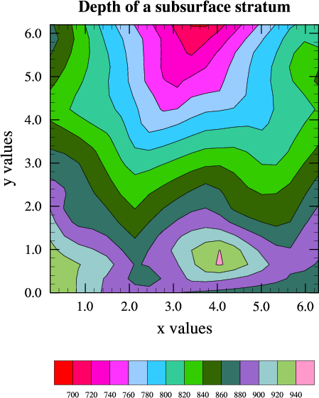
Draw a contour plot of zo, the 2-dimensional array returned from Ngl.natgrid. Label the axes of the contour plot, fill the contour levels, and put a label bar at the bottom.
  resources.sfXArray              = xo            # X axes data points
  resources.sfYArray              = yo            # Y axes data points
Set some ScalarField resources so that the X and Y axis values are the values of the output grid that you defined, rather than index values (which is the default).
  resources.tiMainString          = "Depth of a subsurface stratum"
  resources.tiMainFont            = "Times-Bold"
  resources.tiXAxisString         = "x values"    # X axis label.
  resources.tiYAxisString         = "y values"    # Y axis label.
Set some resources for putting a title at the top of the contour plot and for labeling the X and Y axes. The font for the main title is changed to index 26 ("Times-Bold").
resources.lbOrientation = "Horizontal" # Draw it horizontally.
Since the drawing of a label bar associated with a plot is controlled by the PlotManager, the PlotManager also controls the orientation of it. Thus, use PlotManager resources to change the location of the label bar.
resources.nglSpreadColors = False # Do not interpolate color space.
The "spread colors" feature is turned off so that we get a one-to-one matching between color indices and contour levels.
resources.vpYF = 0.9 # Change Y location of plot.
Drawing a label bar at the bottom causes the plot to go out of the viewport window in this case, so adjust the Y position of the plot on the viewport.
zt = numpy.transpose(zo)
Since Ngl.natgrid returns zo(i,j) as the interpolated value at the coordinate (x(i),y(j)) for 0 < i < numxout and 0 < j < numyout. For the purpose of drawing a contour plot, however, PyNGL identifies the fastest varying dimension (the second dimension of a 2-dimensional array) with the Cartesian X-axis. So, if it is desired to have the x values along the Cartesian X-axis, you need to swap the x and y indices before contouring.
contour = Ngl.contour(xwks,zt,resources)
Note on setting fonts: All the fonts in this contour plot (except the title font) are "Times-Roman." By using a resource file called "ngl08p.res" containing the single entry:
*Font : Times-Roman
you are able to set the font to "Times-Roman" for all
characters drawn in the plot. Any resources that you set within
the PyNGL script override what is set in a resource file. For
example, in you set tiMainFont
above to "Times-Bold," so this font is used for the main title
instead of "Times-Roman". The name of the resource file must
have the same name as the second string passed to Ngl.open_wks, with a ".res" appended.By default, PyNGL looks for the resource file in the same directory as where the script is being executed. If you want to change this default directory, then read the section on resource files. Also, as noted in this section, when you set resources in a resource file, don't put double quotes around predefined strings. Use double quotes only when you actually want the quotes to be part of the string itself.
A more detailed resource file is used in example 9.
#----------- Begin second plot -----------------------------------------
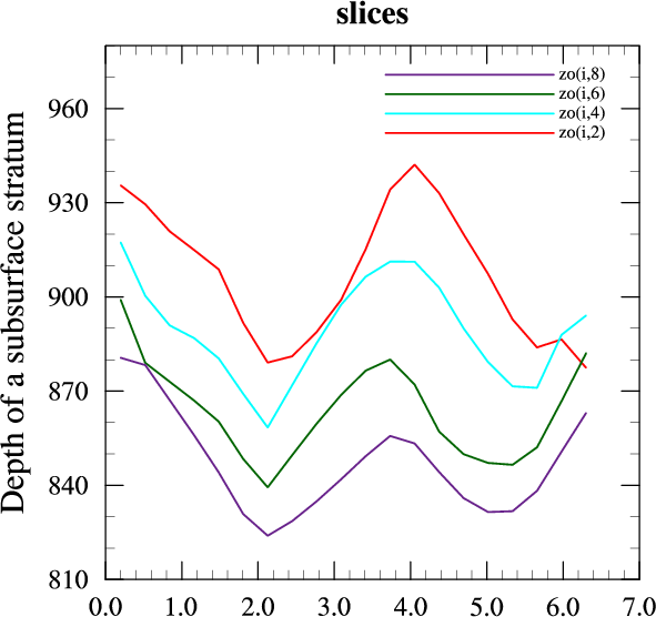
Take some slices of the 2-dimensional zo data and generate an XY plot with four of these slices.
del resources
Since you previously used the resources variable to define some ContourPlot resources, you need to start with a new list of resources for the XyPlot resources, and thus should delete the variable before redefining it.
  resources.xyLineColors        = [2,8,10,14]    # Define line colors.
  resources.xyLineThicknessF    = 3.0             # Define line thickness.
Set some XY plot resources to define the line colors and thickness for each line.
  resources.pmLegendDisplayMode    = "Always"     # Turn on the drawing
  resources.pmLegendZone           = 0            # Change the location
  resources.pmLegendOrthogonalPosF = 0.31         # of the legend
  resources.lgJustification        = "BottomRight"
  resources.pmLegendWidthF         = 0.4          # Change width and
  resources.pmLegendHeightF        = 0.12         # height of legend.
  resources.pmLegendSide           = "Top"        # Change location of
  resources.lgPerimOn              = False        # legend and turn off
Turn on the drawing of a legend. By default, the legend is centered below the plot. To draw the legend in the upper right corner and inside the XY plot, you need to use PlotManager resources to control where the legend is drawn.
By default, the legend appears outside the plot. If you set pmLegendZone to 0, then this allows you to put the legend inside the plot. Setting the resources pmLegendOrthogonalPosF, pmLegendSide, and lgJustification to 0.31, "Top", and "BottomRight", respectively moves the legend to the inside upper right corner of the XY plot.
Legend resources start with "lg" and are defined in the Legend resource descriptions section.
resources.xyExplicitLegendLabels = ["zo(i,2)","zo(i,4)","zo(i,6)","zo(i,8)"]
Set this resource to define labels for the four curves in the legend.
  resources.vpYF      = 0.90  # Change size and location of plot.
  resources.vpXF      = 0.18
  resources.vpWidthF  = 0.74
  resources.vpHeightF = 0.74
Adjust the size and location of the plot so it doesn't run out of the viewport.
resources.trYMaxF = 980 # Set the maximum value for the Y axes.
Change the maximum value of the upper bound of the Y axis to 980.0. The actual maximum of the data is 942.131, which you can verify with print zo. This is done to allow room for the legend you created above to fit inside the top of the plot.
xy = Ngl.xy(xwks,xo,zt[2:9:2,:],resources) # Draw an XY plot.
To pass multiple curves to Ngl.xy, you must pass a 2-dimensional array where the first dimension is the number of curves and the second dimension is the number of points. Assuming that each point of zo is represented by zo(i,j) and that you want to take slices of the data at j = 2, 4, 6, and 8 for all i, then use the transposed array zt with the syntax (2:9:2,:).
#----------- Draw to other workstations ------------------------------
So far in this script you have drawn the graphical output to an X11 workstation. Now draw the contour and XY plot to the other workstations that you opened above.
  Ngl.change_workstation(contour,cgmwks)   # Change the workstation that the
  Ngl.change_workstation(xy,cgmwks)        # contour and XY plot is drawn to.
  Ngl.draw(contour)                        # Draw the contour plot to the new
  Ngl.frame(cgmwks)                        # workstation and advance the frame.
  Ngl.draw(xy)                             # Draw the XY plot to the new
  Ngl.frame(cgmwks)                        # workstation and advance the frame.
To draw the contour and XY plot to the NCGM workstation that you opened, you need to change the current workstation to the NCGM workstation, and then redraw the plots and advance the frame. The Ngl.* plotting functions call Ngl.draw and Ngl.frame for you (unless otherwise specified), so that's why you didn't need to call Ngl.draw and Ngl.frame when the plots were drawn to the X11 window (via the calls to Ngl.contour and Ngl.xy).
Call the procedure Ngl.change_workstation to change the workstation being drawn to. The first argument is the plot that you want to draw (returned from a previous call to one of the Ngl.* plotting functions), and the second argument is the new workstation you want to draw the plot to (returned from a previous call to Ngl.open_wks).
After you've changed the workstation being drawn to, redraw the plots and advance the frame with calls to Ngl.draw and Ngl.frame. If you don't call Ngl.frame after you call Ngl.draw, then the two plots are drawn in the same frame, one on top of the other.
The name of the NCGM file is the second string that you passed to the call to Ngl.open_wks, with the suffix ".ncgm" appended. In this case, the NCGM file name is "ngl08p.ncgm". If you pass an empty string for the second argument to Ngl.open_wks, then the NCGM file is named "nglapp.ncgm".
For information on how to view and edit the NCGM file, see "Viewing and editing your CGMs and raster images". If you are running under X Windows, then you can quickly view your NCGM file with the following command:
ctrans -d X11 name.ncgmAfter the first frame is drawn, click on it with the left mouse button to advance the frame or to exit ctrans.
  Ngl.change_workstation(contour,pswks)  # Do the same for the PostScript
  Ngl.change_workstation(xy,pswks)       # workstation.
  Ngl.draw(contour)
  Ngl.frame(pswks)
  Ngl.draw(xy)
  Ngl.frame(pswks)
To draw the plots to the PostScript workstation that you opened, do the same thing that you did for the NCGM workstation. The name of the PostScript file is the second string that you passed to the call to Ngl.open_wks, with the suffix ".ps" appended. In this case, the PostScript file name is "ngl08p.ps". If you pass an empty string for the second argument to Ngl.open_wks, then the PostScript file is named "nglapp.ps".
  Ngl.change_workstation(contour,pdfwks)  # And for the PDF workstation...
  Ngl.change_workstation(xy,pdfwks)
  Ngl.draw(contour)
  Ngl.frame(pdfwks)
  Ngl.draw(xy)
  Ngl.frame(pdfwks)
To draw the plots to the PDF workstation that you opened, do the same thing that you did for the NCGM and PS workstations.